Exercise - Wolves

Background

Dr. Kevin Schanning used a mail survey designed to measure Michigan, Minnesota, and Wisconsin residents’ feelings, attitudes, experiences with, concerns about management techniques, and knowledge of wolves specific to their state. The survey was 13 pages long, in booklet form, and consisted of 220 questions divided among eight sections: experience with wolves, activities, safety concerns, attitudes, knowledge of wolves in their state, management issues, background (demographics), and how they get their information about wolves. Schanning’s data was recorded in StateOfWolf.csv.

These data are loaded below and reduced to many fewer variables (use of select()) and only those respondents that answered all of those questions (use of complete.cases() within filter()) to reduce the overall size of the data.frame in R. In addition, for the purposes of this exercise, the data.frame was reduced to only those respondents that deer hunted the previous year (i.e., the last filter()). Several variables were converted to groupings with the levels controlled to a proper order (i.e., levels= within factor() within mutate()).¹

library(tidyverse)
lvls_agree <- c("Strongly Disagree","Disagree","Neutral","Agree","Strongly Agree")

#!# Set to your own working directory and have just your filename below.
sow <- read.csv("https://raw.githubusercontent.com/droglenc/NCData/master/StateOfWolf.csv") %>%
  select(state,hunt_deer,seen_wolf,part_deer,
         ad_healthy_deer,ad_nowolves_deer,ad_threaten_deer,ad_deer_hunting) %>%
  filter(complete.cases(.)) %>%
  mutate(part_deer=factor(part_deer,
          levels=c("Stop Participating","Participate Less Frequently",
                   "Participate More Frequently","No Changes")),
         ad_healthy_deer=factor(ad_healthy_deer,levels=lvls_agree),
         ad_nowolves_deer=factor(ad_nowolves_deer,levels=lvls_agree),
         ad_threaten_deer=factor(ad_threaten_deer,levels=lvls_agree),
         ad_deer_hunting=factor(ad_deer_hunting,levels=lvls_agree)) %>%
  filter(hunt_deer=="Yes")

The specific questions with respect to the variable names are as follows:

• state: Resident’s state of residence.
• hunt_deer: Whether or not the respondent hunted deer the previous year (should all be Yes).
• seen_wolf: Whether or not the respondent has ever seen a wolf.
• part_deer: Respondent’s answer to the question “If I knew wolves lived where I participated in deer hunting, I would [‘Stop Participating’, ‘Participate Less Frequently’, ‘Participate More Frequently’, or make ‘No Changes’].”
• ad_healthy_deer: Respondent’s answer to the question “State your level of agreement with the statement ‘Wolves help keep deer herds healthy by killing the sick and the weak animals’.”
• ad_nowolves_deer: Respondent’s answer to the question “State your level of agreement with the statement ‘I think the elimination of wolves from most of the United States has resulted in overabundant and unhealthy deer populations in many places’.”
• ad_threaten_deer: Respondent’s answer to the question “State your level of agreement with the statement ‘The state’s wolf population threatens deer hunting opportunities’.”
• ad_deer_hunting: Respondent’s answer to the question “State your level of agreement with the statement ‘There is no way sportsmen can have good deer hunting if wolves live in the same area’.”

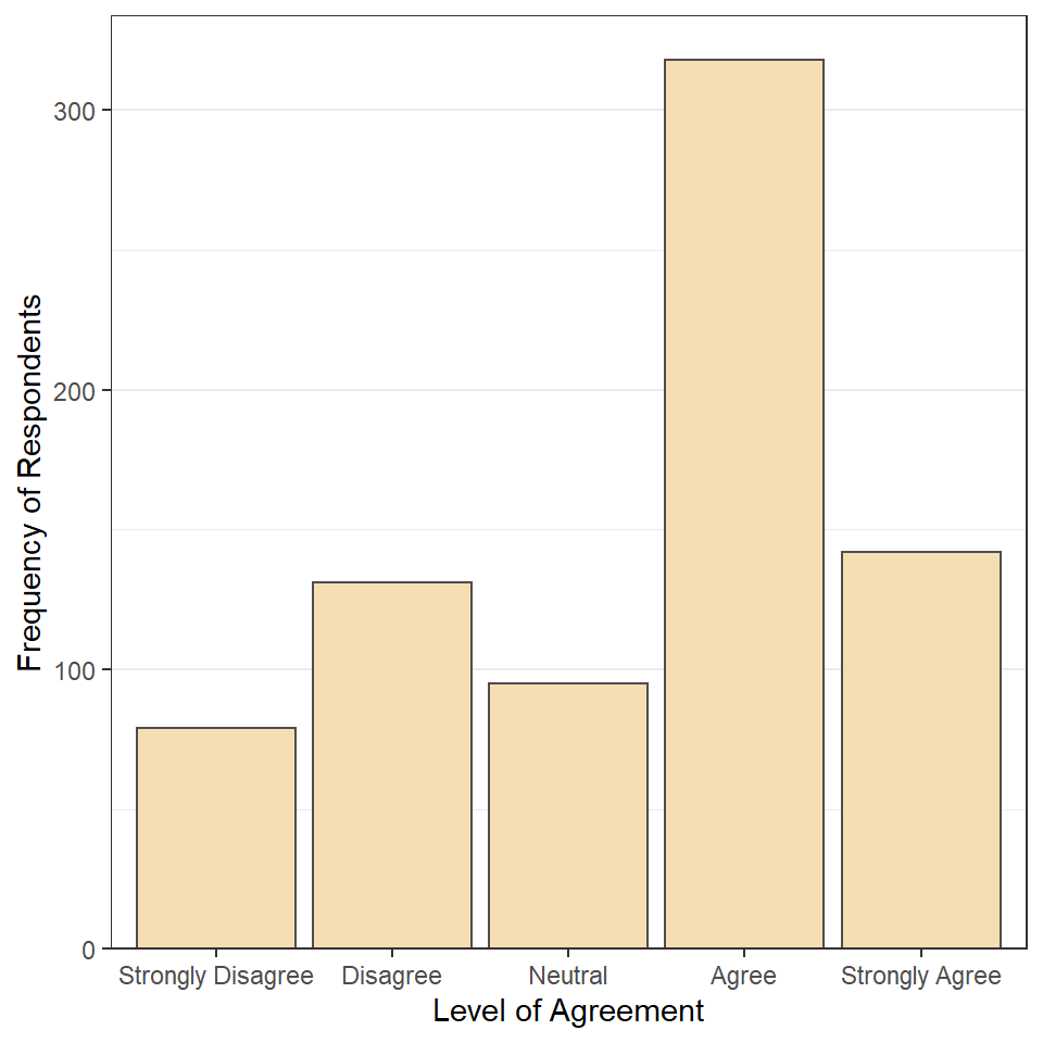
No Good Deer Hunting 1

Construct ggplot2 code to match the graph below (as closely as you can).

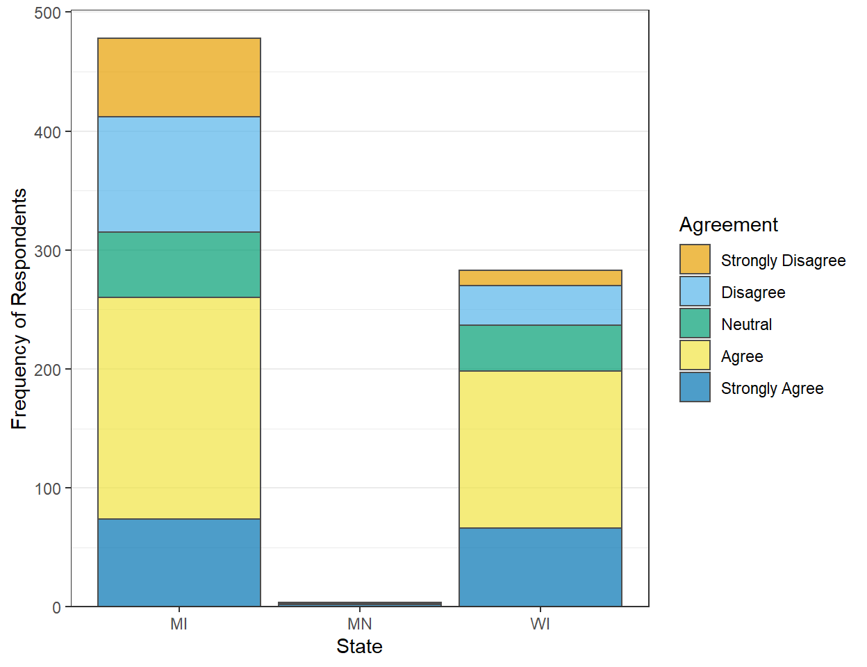
State and No Good Deer Hunting 1

Construct ggplot2 code to match the graph below (as closely as you can … you don’t have to match my colors, but do use other than the default colors).

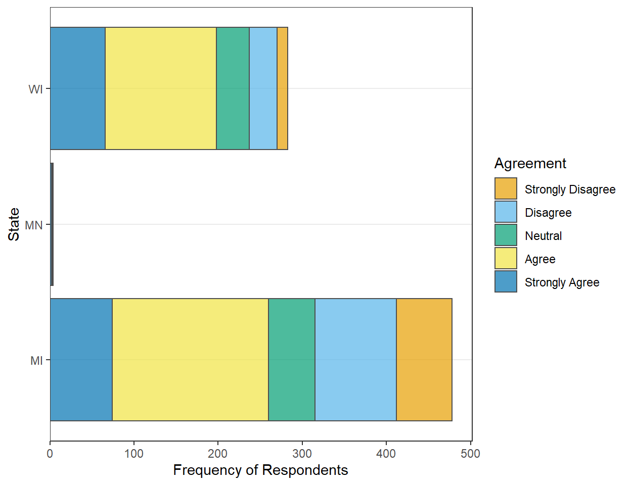
State and No Good Deer Hunting 2

Construct ggplot2 code to match the graph below (as closely as you can).

No Good Deer Hunting 2

Recreate the plot in the “Region 1” section but using summarized data (i.e., summarize the data first and then use that to construct the plot).

State and No Good Deer Hunting 3

Recreate the plot in “State and No Good Deer Hunting 2” using summarized data. [Hint: you will be asked to use percentages in the next section, so you should prepare your summaries here for that.]

## `summarise()` has grouped output by 'state'. You can override using the `.groups` argument.

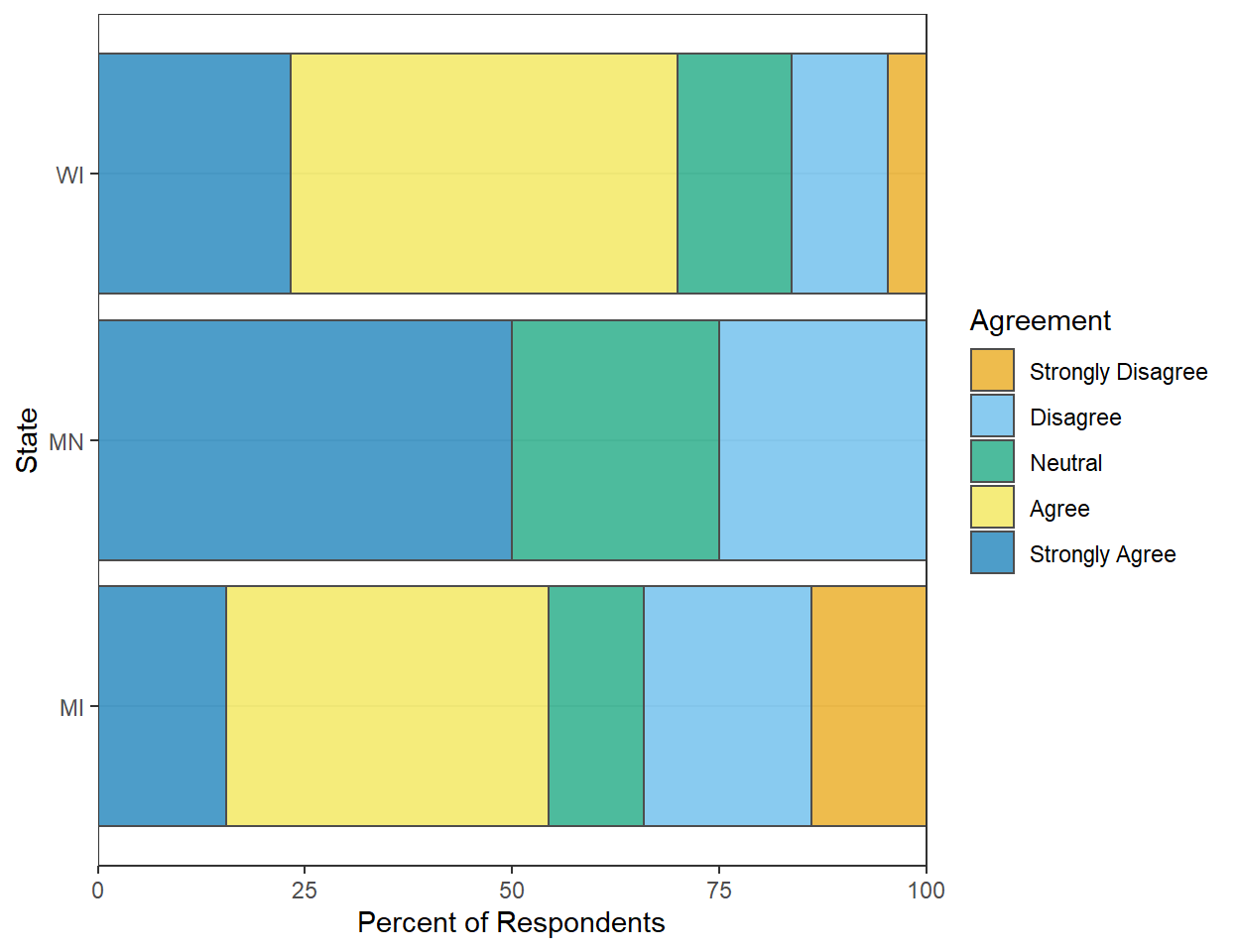
State and No Good Deer Hunting 4

Construct ggplot2 code to match the graph below (as closely as you can).