Background
sports-reference.com has a wealth of information on major American sports. Statistics for Major League Baseball (MLB) players during the 2019 season, which are in this file, will be explored in this exercise.1
These data are loaded below and were restricted to only a few variables (use of select()), those players that had at least 200 at-bats in one league (use of filter()), and were in the top 100 with respect to batting “average” (use of top_n()). In addition, an age-group variable was created (use of case_when() within mutate()) and the Lg and Age_grp variables were converted to groupings (use of factor() within mutate()).2
library(tidyverse)

#!# Set to your own working directory and have just your filename below.
mlb <- read.csv("https://raw.githubusercontent.com/droglenc/NCData/master/MLB19_Batting.csv",
                stringsAsFactors=FALSE) %>%
  select(Name,Age,Lg,G,AB,H,HR,RBI,BB,BA) %>%
  filter(Lg!="MLB",AB>200) %>%  # >200 at-bats in one league
  top_n(n=100,wt=BA) %>%        # players in top 100 by batting average
  mutate(Age_grp=case_when(     # create age groups
    Age < 24 ~ "<24 yrs",
    Age < 30 ~ "24-30 yrs",
    TRUE ~ ">30 yrs"),
    Age_grp=factor(Age_grp,levels=c("<24 yrs","24-30 yrs",">30 yrs")),
    Lg=factor(Lg))
str(mlb)
Here we will only use the following variables:
BA: Batting average (as a proportion).Lg: League competed in (ALorNL).Age_grp: Age grouping (<24 yrs,24-30 yrs,>30 yrs).
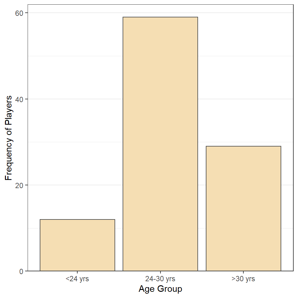
Age Groups 1
Construct ggplot2 code to match the graph below (as closely as you can).
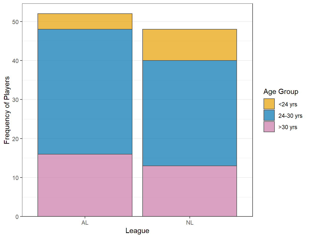
League and Age Group 1
Construct ggplot2 code to match the graph below (as closely as you can … you don’t have to match my colors, but do use other than the default colors).
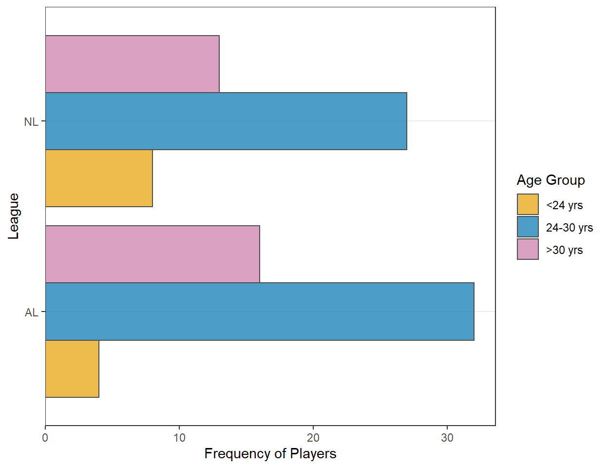
League and Age Group 2
Construct ggplot2 code to match the graph below (as closely as you can).
Age Group 2
Recreate the plot in the “Region 1” section but using summarized data (i.e., summarize the data first and then use that to construct the plot).
League and Age Group 3
Recreate the plot in “League and Age Group 2” using summarized data. [Hint: you will be asked to use percentages in the next section, so you should prepare your summaries here for that.]
## `summarise()` has grouped output by 'Lg'. You can override using the `.groups` argument.
League and Age Group 4
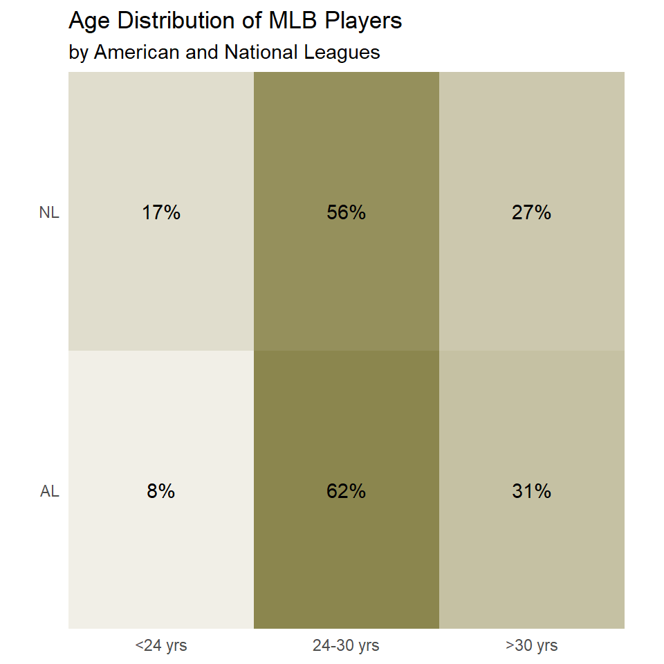
Construct ggplot2 code to match the graph below (as closely as you can).
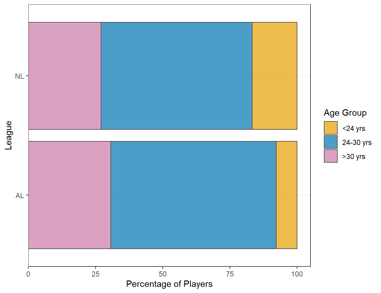
League and Age Group 5
Construct ggplot2 code to match the graph below (as closely as you can).
Footnote
These data were obtained from https://www.sports-reference.com/ with the following steps: 1) Select “Baseball” in the list of sports in the gray box near the top of the page; 2) Select “Seasons” in the list of items in the gray box near the top of the page; 3) Select “Batting” after “All Major Leagues” under “League Index”, 4) Select “2019” in the list of years; 5) Scroll down to “Player Standard Batting”; 6) hover over the “Share & more” item just after “Player Standard Batting” above the table of statistics and select “Get Table as a CSV”; and 7) copy CSV result to a text file.↩︎
These code can be copied as is, but make sure to set your working directory with
setwd()and to put just the filename insideread.csv().↩︎