Background
Lake Erie is world-renowned for its Walleye [Sander vitreus] population and fishing. The Ohio Department of Natural Resources samples Walleye with gillnets from three regions of Lake Erie every fall. Their results from 2003-2014 are stored in this file from the fishR webpage. Metadata for this file is here. The data are loaded below1 and, for this exercise, reduced to only those fish captured in 2003 (i.e., filter()), the location codes are changed from numbers to words (i.e., mapvalues() within mutate()), and location is converted groupings (i.e., factor() within mutate()).2
#!# Set to your own working directory and have just your filename below.
wae <- read.csv("https://raw.githubusercontent.com/droglenc/FSAdata/master/data-raw/WalleyeErie2.csv") %>%
  filter(year==2003) %>%
  mutate(loc=plyr::mapvalues(loc,from=c(1,2,3),
              to=c("Toledo-Huron","Huron-Fairport","Fairport-Conneaut")),
         loc=factor(loc))
str(wae)
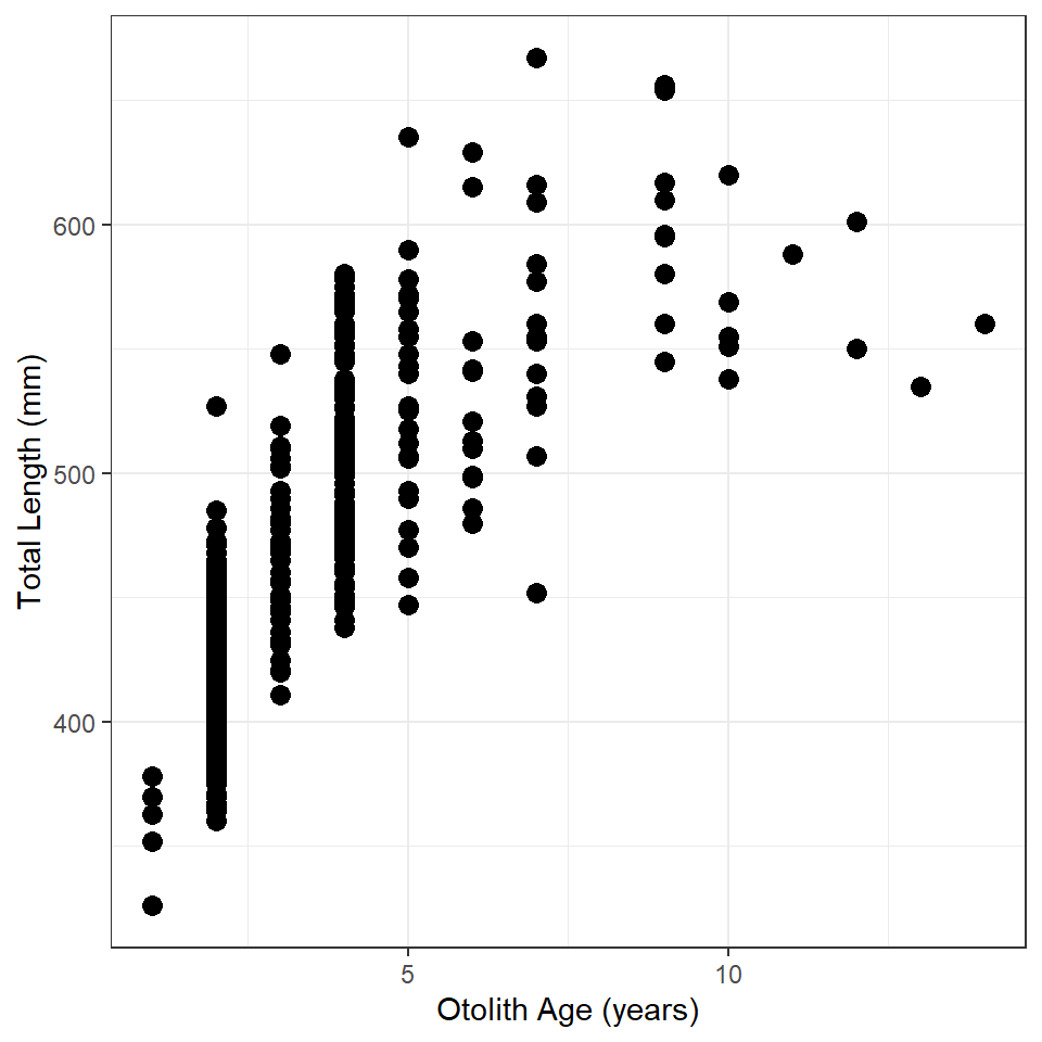
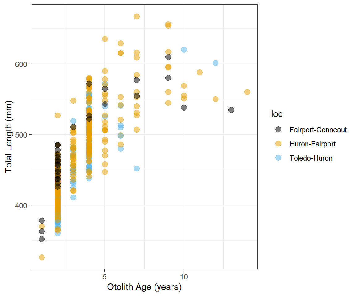
Total Length vs Age 1
Construct ggplot2 code to match the graph below (as closely as you can).
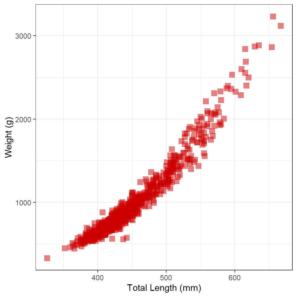
Weight vs Total Length
Construct ggplot2 code to match the graph below (as closely as you can). [HINT: The graphic at the bottom of this page might be useful.]
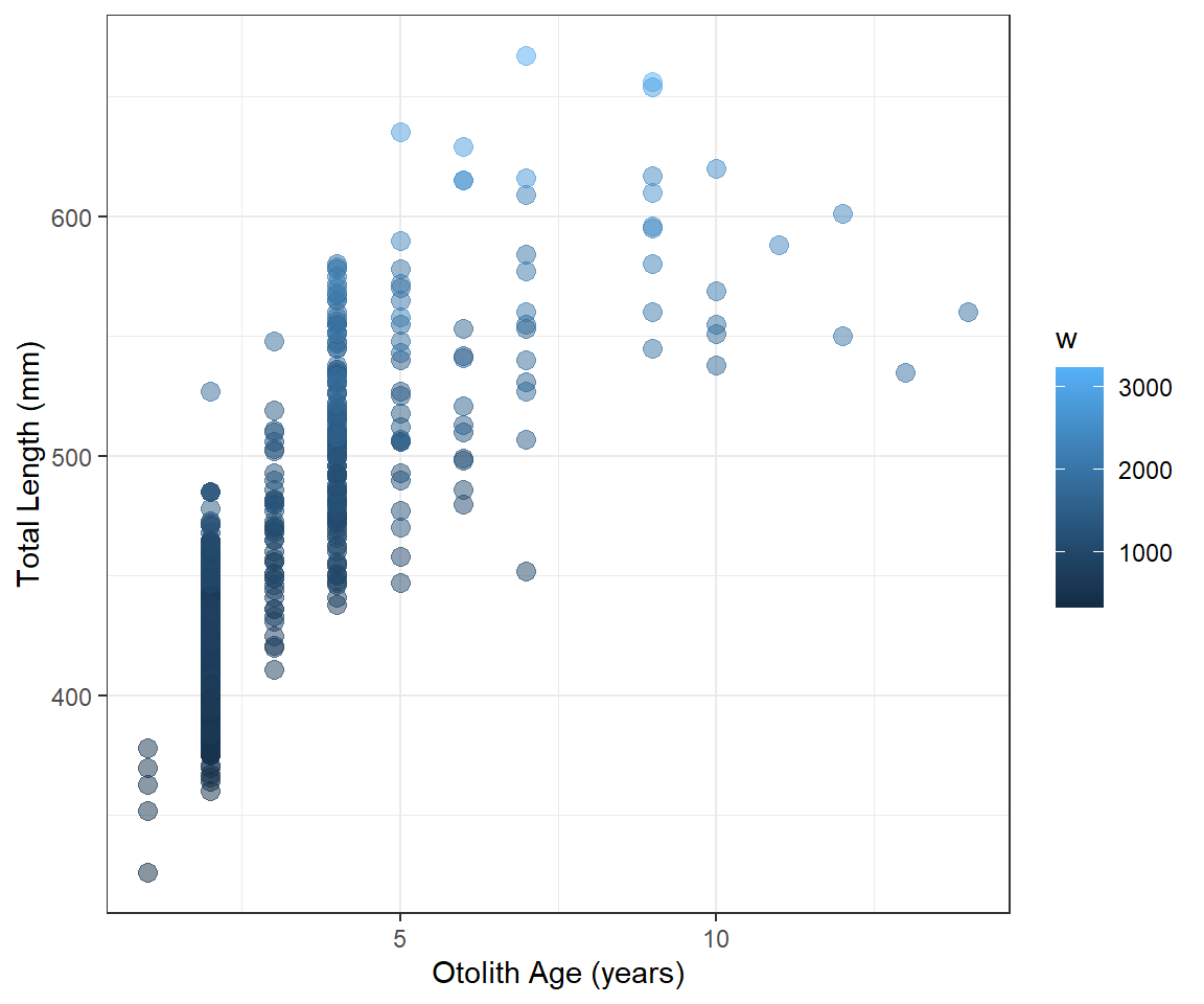
Total Length vs Age 2
Construct ggplot2 code to match the graph below (as closely as you can).

Total Length vs Age 3
Construct ggplot2 code to match the graph below (as closely as you can).
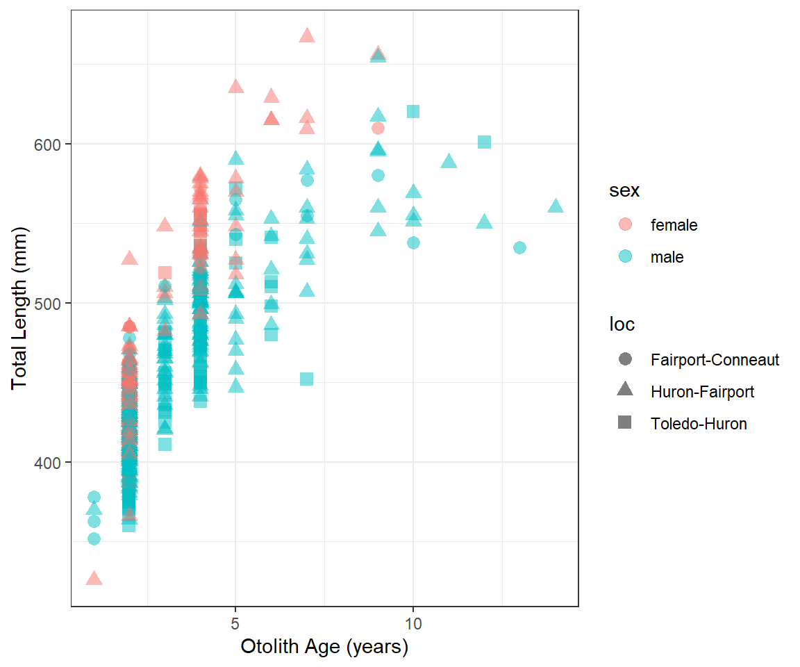
Total Length vs Age 4
Construct ggplot2 code to match the graph below (as closely as you can).
Total Length vs Age 5
Modify your plot from “Total Length vs Age 2” to use three divergent colors for the different locations that are colorblind-safe. See the color brewer website or these color-blind-friendly pallettes for help with this. Note that hexadecimal codes for colors can be entered the same as names of colors.
These data were read directly from the webpage. However, the data can be downloaded to your computer and loaded from there into R, which would be similar to how you would load your own data into R. How to load a CSV file into RStudio is described in this video, for which the password is “NCStats” (without the quotes).↩︎
These code can be copied as is, but make sure to set your working directory with
setwd()and to put just the filename insideread.csv().↩︎