Background
The National Oceanic and Atmospheric Administration (NOAA) maintains a database of global land and sea temperatures. The data can be accessed from their Climate at a Glance website. Their default settings show the global temperature anomaly (difference from a long-term average) for February and are in this CSV file. The data file is loaded into R below,1 but note that skip=4 is need as the first four lines of the CSV file do not contain data.2
#!# Set to your own working directory and have just your filename below.
gt <- read.csv("https://www.ncdc.noaa.gov/cag/global/time-series/globe/land_ocean/1/2/1880-2020/data.csv",skip=4)
str(gt)
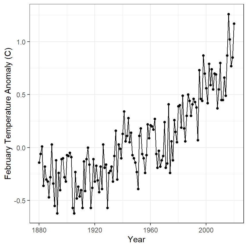
Annual Temperature Anomaly 1
Construct ggplot2 code to match the graph below (as closely as you can).
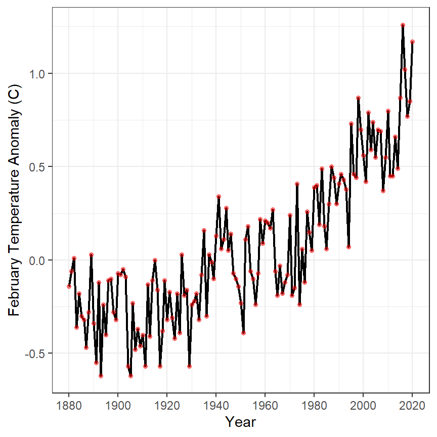
Annual Temperature Anomaly 2
Construct ggplot2 code to match the graph below (as closely as you can). [HINT: Copy and then modify the code you constructed from above.]
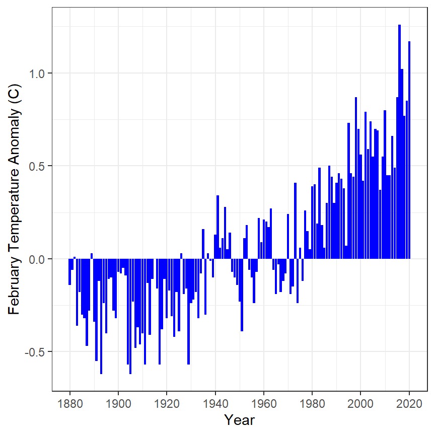
Annual Temperature Anomaly 3
Construct ggplot2 code to match the graph below (as closely as you can).
BONUS – Annual Temperature Anomaly 4
Perform an internet search to determine how to add a solid black horizontal line at 0 to each of the graphs above (see the line in the graph in the next section).
BONUS – Annual Temperature Anomaly 5
Construct ggplot2 code to match the graph below (as closely as you can).
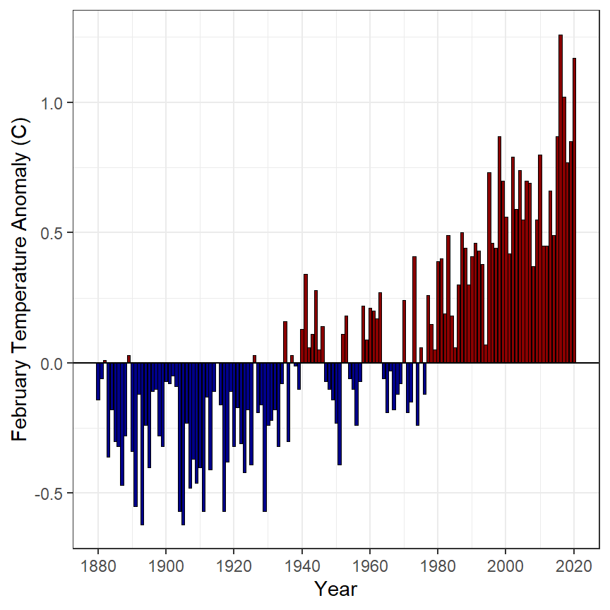
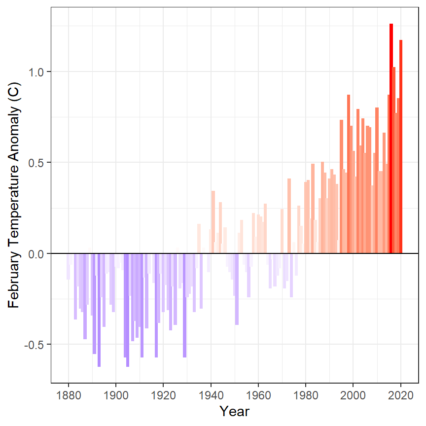
BONUS – Annual Temperature Anomaly 6
Construct ggplot2 code to match the graph below (as closely as you can).
These data were read directly from the webpage. However, the data can be downloaded to your computer and loaded from there into R, which would be similar to how you would load your own data into R. How to load a CSV file into RStudio is described in this video, for which the password is “NCStats” (without the quotes).↩︎
These code can be copied as is, but make sure to set your working directory with
setwd()and to put just the filename insideread.csv().↩︎