Background
sports-reference.com has a wealth of information on major American sports. Statistics for college quarterbacks from the 2019-20 season, which were saved into NCAAF19_QBS.csv, will be explored in this exercise.1
Perform the following steps to load the data for all quarterbacks from the 2019-20 season,2 restrict the data to only those in the so-called “power 5 conferences” (i.e., filter()), and make sure that the Conference variable is a grouping variable (i.e., factor()).3
#!# Set to your own working directory and have just your filename below.
qbs <- read.csv("https://raw.githubusercontent.com/droglenc/NCData/master/NCAAF19_QBS.csv",
                stringsAsFactors=FALSE) %>%
  filter(Conf %in% c("ACC","Big 12","Big Ten","Pac-12","SEC")) %>%
  mutate(Conf=factor(Conf))
str(qbs)
Here we will only use the following variables:
Conf: Conference team played in.Int: Total number of interceptions.Y_A: Number of yards per passing attempt.Att: Number of attempted passes.Ratt: Number of attempted rushes (i.e., runs).Pct: Percentage of attempted passes that were completed.
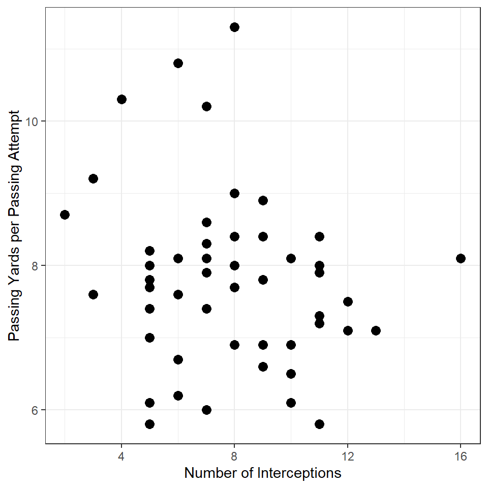
Passing Efficiency vs. Interceptions
Construct ggplot2 code to match the graph below (as closely as you can).
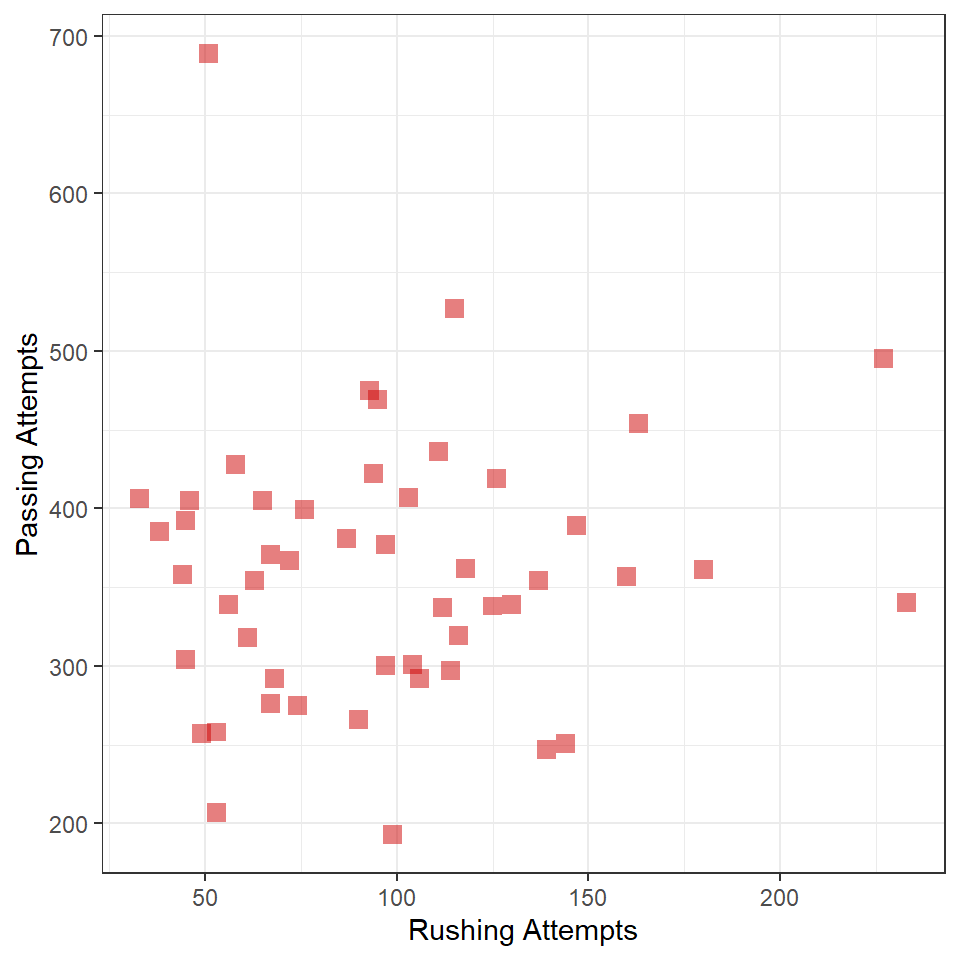
Passing Attempts vs Rushing Attempts 1
Construct ggplot2 code to match the graph below (as closely as you can). [HINT: The graphic at the bottom of this page might be useful.]
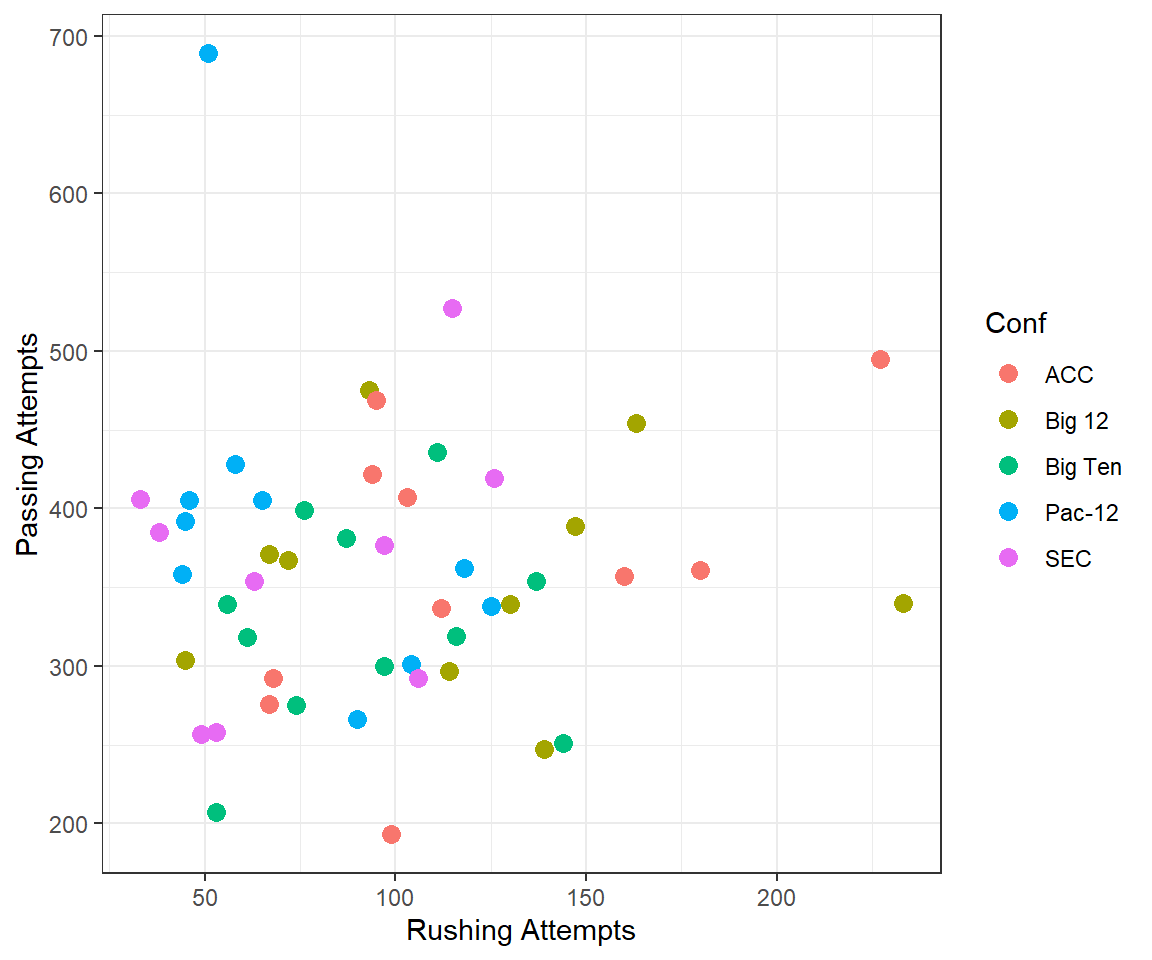
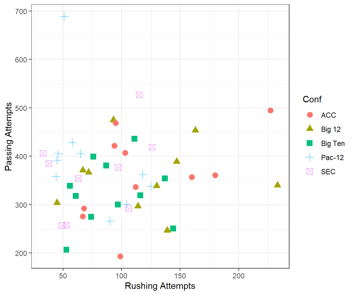
Passing Attempts vs Rushing Attempts 2
Construct ggplot2 code to match the graph below (as closely as you can).
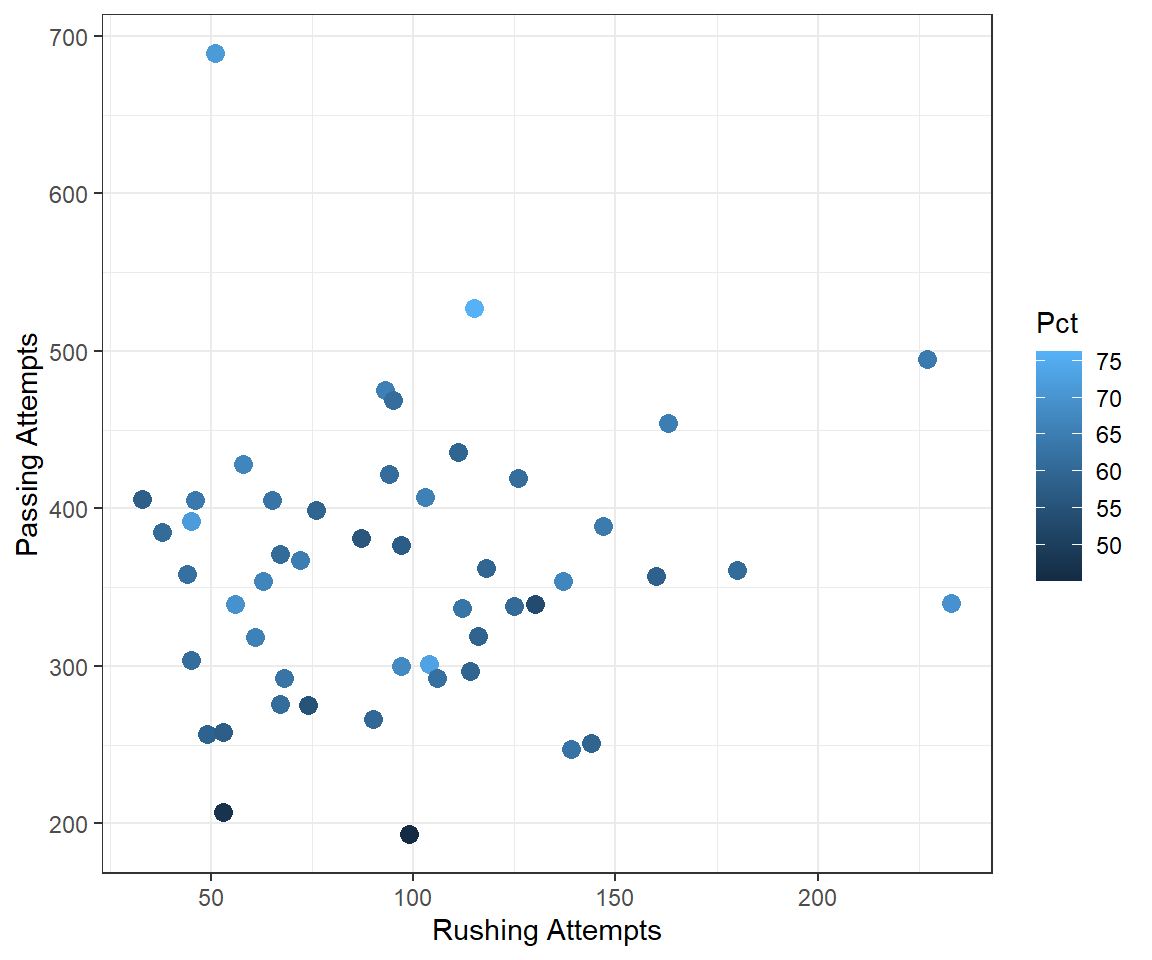
Passing Attempts vs Rushing Attempts 3
Construct ggplot2 code to match the graph below (as closely as you can).
Passing Attempts vs Rushing Attempts 4
Construct ggplot2 code to match the graph below (as closely as you can).
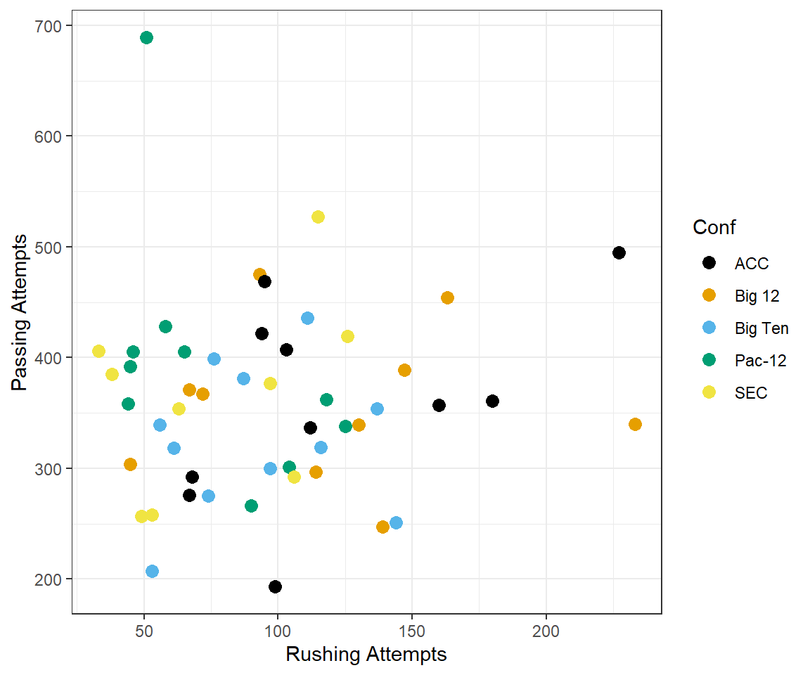
Passing Attempts vs Rushing Attempts 5
Modify your plot from “Passing Attempts vs Rushing Attempts 2” to use five divergent colors for the different conferences that are colorblind-safe. See the color brewer website or these color-blind-friendly pallettes for help with this. Note that hexadecimal codes for colors can be entered the same as names of colors.
These data were obtained from https://www.sports-reference.com/ with the following steps: 1) Select “CFB” in the list of sports in the gray box near the top of the page; 2) Select “Years” in the list of items in the gray box near the top of the page; 3) Select “2019” in the list of years; 4) Hover over “Stats” in the gray box near the middle of the page and select “Passing” from the items that will appear; 5) Hover over the “Share & more” item just above the top-right side of the table of statistics and select “Get Table as a CSV”; and 6) copy CSV result to a text file, delete the first line, and slightly modify the variable names.↩︎
These data were read directly from the webpage. However, the data can be downloaded to your computer and loaded from there into R, which would be similar to how you would load your own data into R. How to load a CSV file into RStudio is described in this video, for which the password is “NCStats” (without the quotes).↩︎
These code can be copied as is, but make sure to set your working directory with
setwd()and to put just the filename insideread.csv().↩︎