Background
Dr. Jim Paruk studied the morphology of Common Loons (Gavia immer), primarily their bills, from a wide variety of locations in North America. These data are in Loon1.csv, with information about these data in this metadata file. These data are then loaded into R and their structure examined below.1
## #!# Set to your own working directory and have just your filename below.
loon <- read.csv("https://raw.githubusercontent.com/droglenc/NCData/master/Loon1.csv")
str(loon)
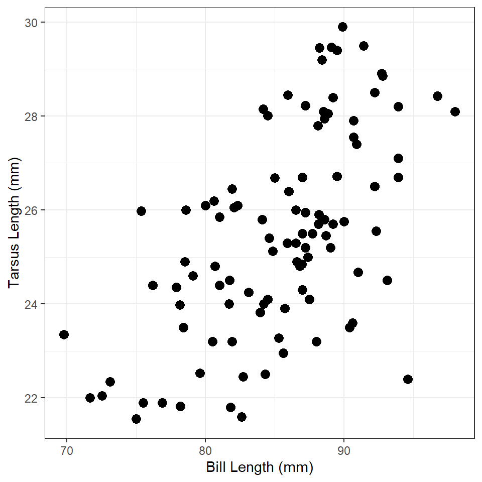
Tarsus Length vs. Bill Length 1
Construct ggplot2 code to match the graph below (as closely as you can).
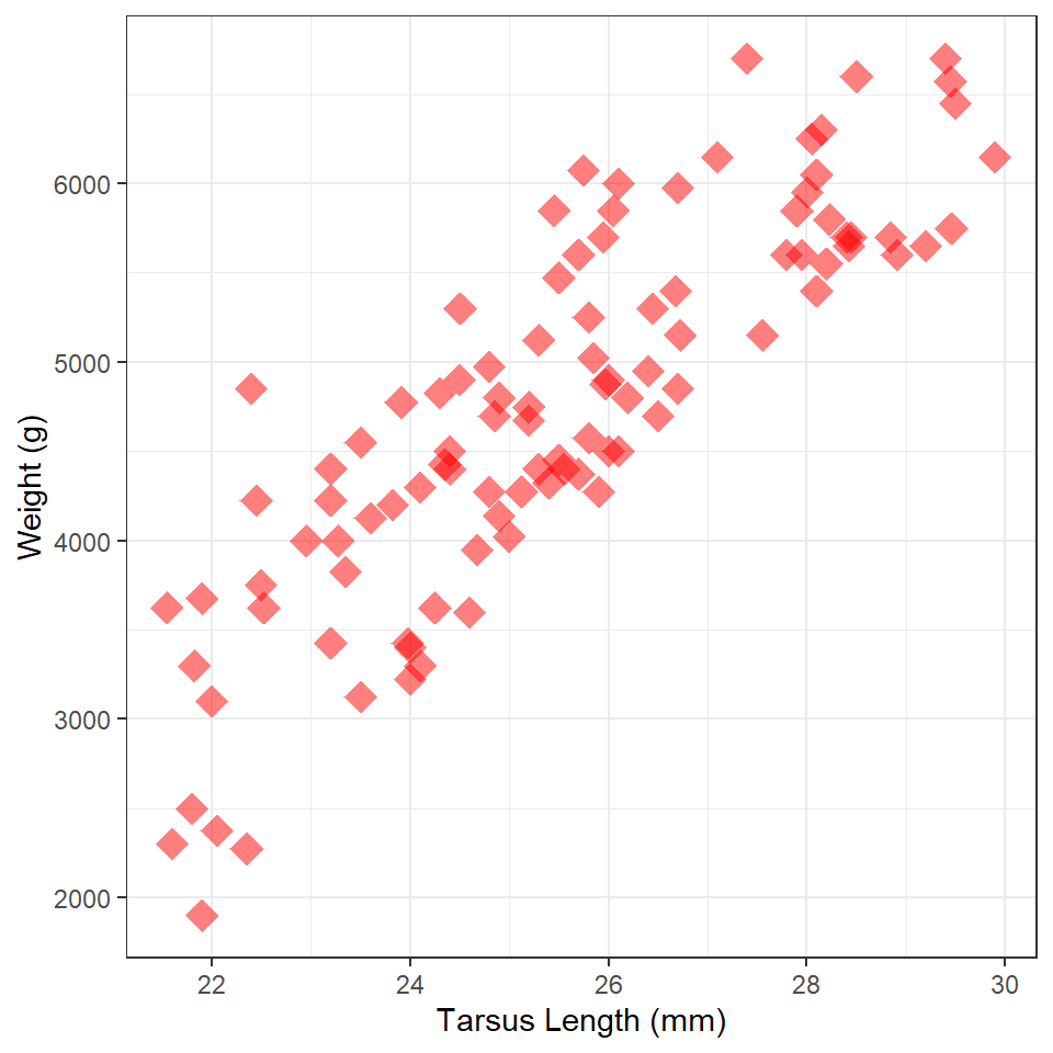
Weight vs Tarsus Length
Construct ggplot2 code to match the graph below (as closely as you can). [HINT: The graphic at the bottom of this page might be useful.]
Tarsus Length vs. Bill Length 2
Construct ggplot2 code to match the graph below (as closely as you can).
Tarsus Length vs. Bill Length 3
Construct ggplot2 code to match the graph below (as closely as you can).
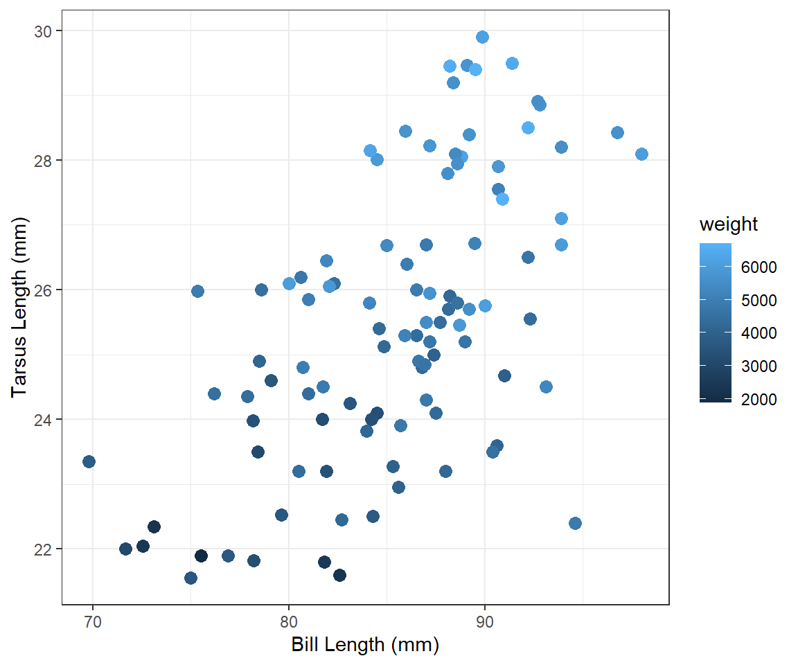
Tarsus Length vs. Bill Length 4
Construct ggplot2 code to match the graph below (as closely as you can).
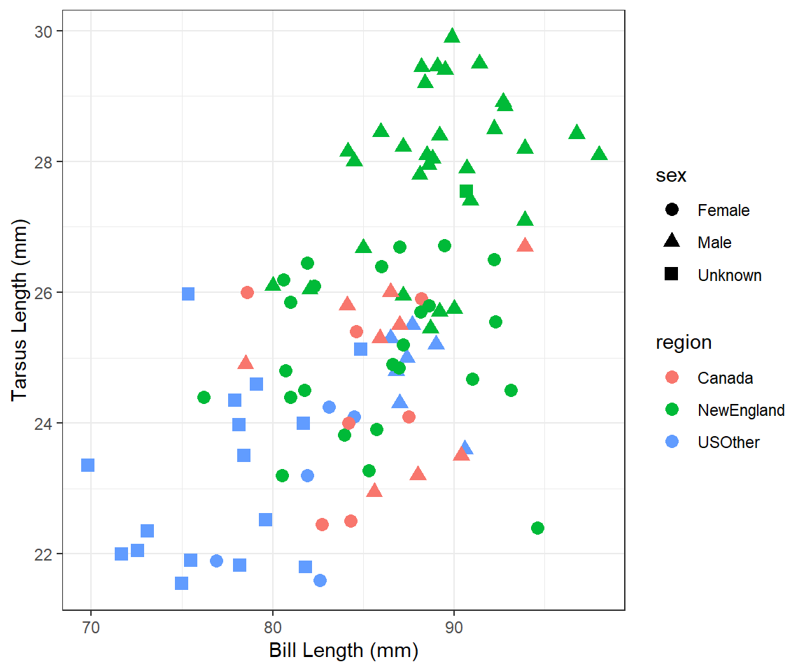
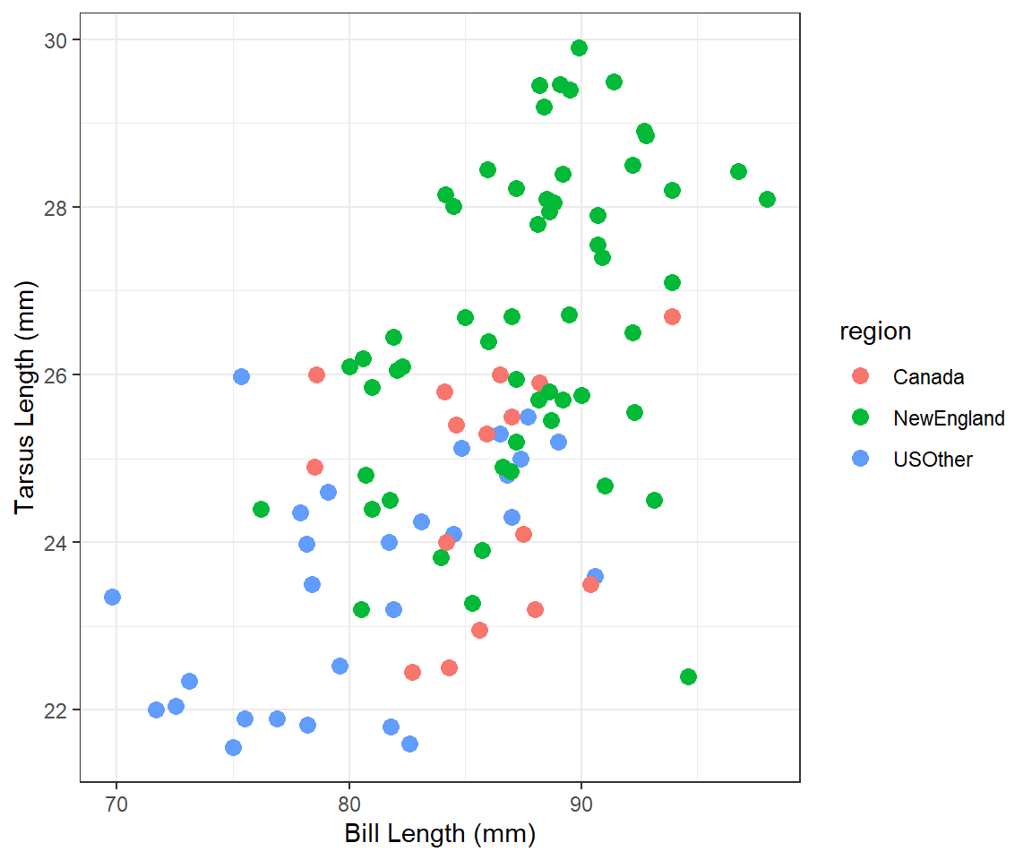
Tarsus Length vs. Bill Length 5
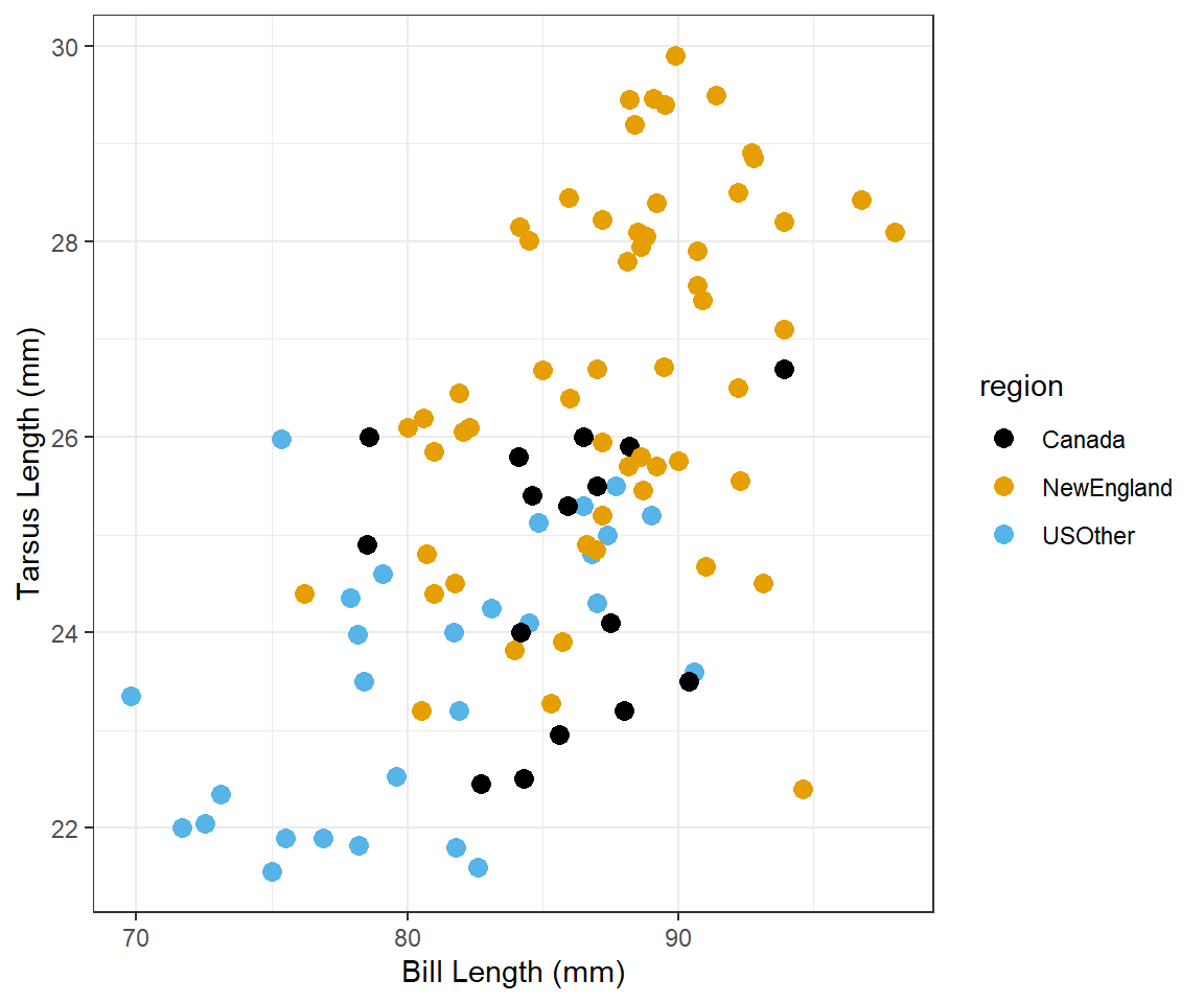
Modify your plot from “Tarsus Length vs Bill Length 2” to use three divergent colors for the different regions that are colorblind-safe. See the color brewer website or these color-blind-friendly palettes for help with this. Note that hexadecimal codes for colors can be entered the same as names of colors.
These data were read directly from the webpage. However, the data can be downloaded to your computer and loaded from there into R, which would be similar to how you would load your own data into R. How to load a CSV file into RStudio is described in this video, for which the password is “NCStats” (without the quotes).↩︎